page 104 of IPCC WG1 AR5
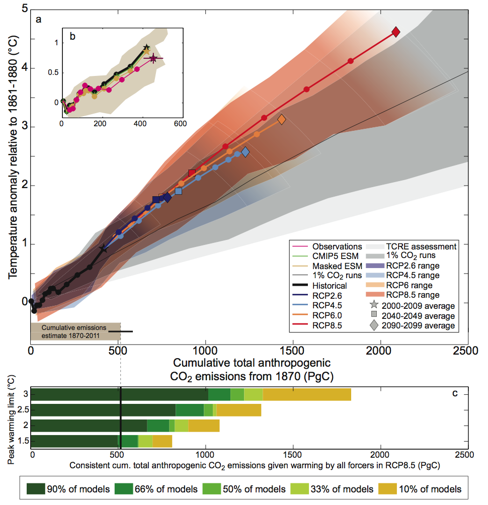
TFE.8, Figure 1 | Global mean temperature increase since 1861-1880 as a function of cumulative total global CO2 emissions from various lines of evidence.
Note that the fraction of models cannot be interpreted as a probability.
The budgets are derived from the RCP8.5 runs, with relative high non-CO2 forcing over the 21st century. If non-CO2 are significantly reduced, the CO2 emissions compatible with a specific temperature limit might be slightly higher, but only to a very limited degree, as illustrated by the other coloured lines in (a), which assume significantly lower non-CO2 forcing. Further detail regarding the related Figure SPM.10 is given in the TS Supplementary Material. {Figure 12.45}
The concept of stabilization is strongly linked to the ultimate objective of the United Nations Framework Convention on Climate Change (UNFCCC), which is ‘to achieve [...] stabilization of greenhouse gas concentrations in the atmosphere at a level that would prevent dangerous anthropogenic interference with the climate system’. Recent policy discussions focused on limits to a global temperature increase, rather than to greenhouse gas (GHG) concentrations, as climate targets in the context of the UNFCCC objectives. The most widely discussed is that of 2°C, that is, to limit global temperature increase relative to pre-industrial times to below 2°C, but targets other than 2°C have been proposed (e.g., returning warming to well below 1.5°C global warming relative to pre-industrial, or returning below an atmospheric carbon dioxide (CO2) concentration of 350 ppm). Climate targets generally mean avoiding a warming beyond a predefined threshold. Climate impacts, however, are geographically diverse and sector specific, and no objective threshold defines when dangerous interference is reached. Some changes may be delayed or irreversible, and some impacts could be beneficial. It is thus not possible to define a single critical objective threshold without value judgements and without assumptions on how to aggregate current and future costs and benefits. This TFE does not advocate or defend any threshold or objective, nor does it judge the economic or political feasibility of such goals, but assesses, based on the current understanding of climate and carbon cycle feedbacks, the climate projections following the Representative Concentration Pathways (RCPs) in the context of climate targets, and the implications of different long-term temperature stabilization objectives on allowed carbon emissions. Further below it is highlighted that temperature stabilization does not necessarily imply stabilization of the entire Earth system. {12.5.4}
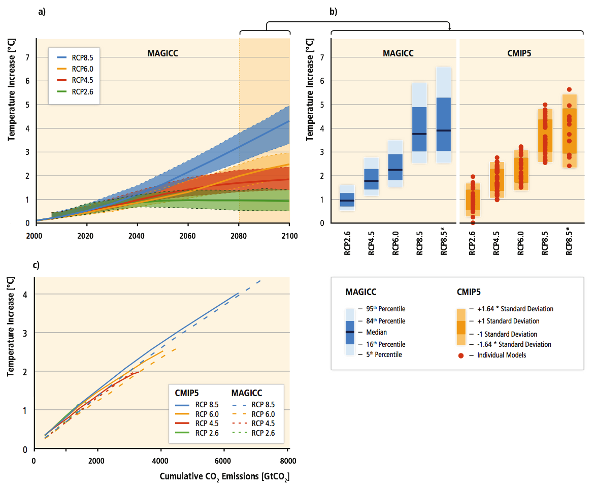
Temperature targets imply an upper limit on the total radiative forcing (RF). Differences in RF between the four RCP scenarios are relatively small up to 2030, but become very large by the end of the 21st century and dominated by CO2 forcing. Consequently, in the near term, global mean surface temperatures (GMSTs) are projected to continue to rise at a similar rate for the four RCP scenarios. Around the mid-21st century, the rate of global warming begins to be more strongly dependent on the scenario. By the end of the 21st century, global mean temperatures will be warmer than present day under all the RCPs, global temperature change being largest (>0.3°C per decade) in the highest RCP8.5 and significantly lower in RCP2.6, particularly after about 2050 when global surface temperature response stabilizes (and declines thereafter) (see Figure TS.15). {11.3.1, 12.3.3, 12.4.1}
In the near term (2016–2035), global mean surface warming is more likely than not to exceed 1°C and very unlikely to be more than 1.5°C relative to the average from year 1850 to 1900 (assuming 0.61°C warming from 1850-1900 to 1986–2005) (medium confidence). By the end of the 21st century (2081–2100), global mean surface warming, relative to 1850-1900, is likely to exceed 1.5°C for RCP4.5, RCP6.0 and RCP8.5 (high confidence) and is likely to exceed 2°C for RCP6.0 and RCP8.5 (high confidence). It is more likely than not to exceed 2°C for RCP4.5 (medium confidence). Global mean surface warming above 2°C under RCP2.6 is unlikely (medium confidence). Global mean surface warming above 4°C by 2081–2100 is unlikely in all RCPs (high confidence) except for RCP8.5 where it is about as likely as not (medium confidence). {11.3.6, 12.4.1; Table 12.3}
Continuing GHG emissions beyond 2100 as in the RCP8.5 extension induces a total RF above 12 W m–2 by 2300, with global warming reaching 7.8 [3.0 to 12.6] °C for 2281–2300 relative to 1986–2005. Under the RCP4.5 extension, where radiative forcing is kept constant (around 4.5 W m-2) beyond 2100, global warming reaches 2.5 [1.5 to 3.5] °C. Global warming reaches 0.6 [0.0 to 1.2] °C under the RCP2.6 extension where sustained negative emissions lead to a further decrease in RF, reaching values below present-day RF by 2300. See also Box TS.7. {12.3.1, 12.4.1, 12.5.1} The total amount of anthropogenic CO2 released in the atmosphere since pre-industrial (often termed cumulative carbon emission, although it applies only to CO2 emissions) is a good indicator of the atmospheric CO2 concentration and hence of the global warming response. The ratio of GMST change to total cumulative anthropogenic CO2 emissions is relatively constant over time and independent of the scenario. This near-linear relationship between total CO2 emissions and global temperature change makes it possible to define a new quantity, the transient climate response to cumulative carbon emission (TCRE), as the transient GMST change for a given amount of cumulated anthropogenic CO2 emissions, usually 1000 PgC (TFE.8, Figure 1). TCRE is model dependent, as it is a function of the cumulative CO2 airborne fraction and the transient climate response, both quantities varying significantly across models. Taking into account the available information from multiple lines of evidence (observations, models and process understanding), the near linear relationship between cumulative CO2 emissions and peak global mean temperature is well established in the literature and robust for cumulative total CO2 emissions up to about 2000 PgC. It is consistent with the relationship inferred from past cumulative CO2 emissions and observed warming, is supported by process understanding of the carbon cycle and global energy balance, and emerges as a robust result from the entire hierarchy of models. Expert judgment based on the available evidence suggests that TCRE is likely between 0.8°C and 2.5°C per 1000 PgC, for cumulative emissions less than about 2000 PgC until the time at which temperature peaks (TFE.8, Figure 1a). {6.4.3, 12.5.4; Box 12.2}
CO2-induced warming is projected to remain approximately constant for many centuries following a complete cessation of emissions. A large fraction of climate change is thus irreversible on a human time scale, except if net anthropogenic CO2 emissions were strongly negative over a sustained period. Based on the assessment of TCRE (assuming a normal distribution with a ±1 standard deviation range of 0.8 to 2.5°C per 1000 PgC), limiting the warming caused by anthropogenic CO2 emissions alone (i.e., ignoring other radiative forcings) to less than 2°C since the period 1861–1880 with a probability of >33%, >50% and >66%, total CO2 emissions from all anthropogenic sources would need to be below a cumulative budget of about 1570 PgC, 1210 PgC and 1000 PgC since 1870, respectively. An amount of 515 [445 to 585] PgC was emitted between 1870 and 2011 (TFE.8, Figure 1a,b). Higher emissions in earlier decades therefore imply lower or even negative emissions later on. Accounting for non-CO2 forcings contributing to peak warming implies lower cumulated CO2 emissions. Non-CO2 forcing constituents are important, requiring either assumptions on how CO2 emission reductions are linked to changes in other forcings, or separate emission budgets and climate modelling for short-lived and long-lived gases. So far, not many studies have considered non-CO2 forcings. Those that do consider them found significant effects, in particular warming of several tenths of a degree for abrupt reductions in emissions of short-lived species, like aerosols. Accounting for an unanticipated release of GHGs from permafrost or methane hydrates, not included in studies assessed here, would also reduce the anthropogenic CO2 emissions compatible with a given temperature target. Requiring a higher likelihood of temperatures remaining below a given temperature target would further reduce the compatible emissions (TFE.8, Figure 1c). When accounting for the non-CO2 forcings as in the RCP scenarios, compatible carbon emissions since 1870 are reduced to about 900 PgC, 820 PgC and 790 PgC to limit warming to less than 2°C since the period 1861–1880 with a probability of >33%, >50%, and >66%, respectively. These estimates were derived by computing the fraction of the Coupled Model Intercomparison Project Phase 5 (CMIP5) Earth System Models (ESMs) and Earth System Models of Intermediate Complexity (EMICs) that stay below 2°C for given cumulative emissions following RCP8.5, as shown in TFE.8 Fig. 1c. The non-CO2 forcing in RCP8.5 is higher than in RCP2.6. Because all likelihood statements in calibrated IPCC language are open intervals, the estimates provided are thus both conservative and consistent choices valid for non-CO2 forcings across all RCP scenarios. There is no RCP scenario which limits warming to 2°C with probabilities of >33% or >50%, and which could be used to directly infer compatible cumulative emissions. For a probability of >66% RCP2.6 can be used as a comparison. Combining the average back-calculated fossil fuel carbon emissions for RCP2.6 between 2012 and 2100 (270 PgC) with the average historical estimate of 515 PgC gives a total of 785 PgC, i.e., 790 PgC when rounded to 10 PgC. As the 785 PgC estimate excludes an explicit assessment of future land-use change emissions, the 790 PgC value also remains a conservative estimate consistent with the overall likelihood assessment. The ranges of emissions for these three likelihoods based on the RCP scenarios are rather narrow, as they are based on a single scenario and on the limited sample of models available (TFE.8 Fig. 1c). In contrast to TCRE they do not include observational constraints or account for sources of uncertainty not sampled by the models. The concept of a fixed cumulative CO2 budget holds not just for 2°C, but for any temperature level explored with models so far (up to about 5°C, see Figures 12.44 to 12.46). Higher temperature targets would allow larger cumulative budgets, while lower temperature target would require lower cumulative budgets (TFE.8, Figure 1). {6.3.1, 12.5.2, 12.5.4}
The climate system has multiple time scales, ranging from annual to multi-millennial, associated with different thermal and carbon reservoirs. These long time scales induce a commitment warming ‘already in the pipe-line’. Stabilization of the forcing would not lead to an instantaneous stabilization of the warming. For the RCP scenarios and their extensions to 2300, the fraction of realized warming, at that time when RF stabilizes, would be about 75 to 85% of the equilibrium warming. For a 1% yr–1 CO2 increase to 2 x CO2 or 4 x CO2 and constant forcing thereafter, the fraction of realized warming would be much smaller, about 40 to 70% at the time when the forcing is kept constant. Owing to the long time scales in the deep ocean, full equilibrium is reached only after hundreds to thousands of years. {12.5.4}
The commitment to past emissions is a persistent warming for hundreds of years, continuing at about the level of warming that has been realized when emissions were ceased. The persistence of this CO2-induced warming after emission have ceased results from a compensation between the delayed commitment warming described above and the slow reduction in atmospheric CO2 resulting from ocean and land carbon uptake. This persistence of warming also results from the nonlinear dependence of RF on atmospheric CO2, that is, the relative decrease in forcing being smaller than the relative decrease in CO2 concentration. For high climate sensitivities, and in particular if sulphate aerosol emissions are eliminated at the same time as GHG emissions, the commitment from past emission can be strongly positive, and is a superposition of a fast response to reduced aerosols emissions and a slow response to reduced CO2. {12.5.4}
Stabilization of global temperature does not imply stabilization for all aspects of the climate system. Processes related to vegetation change, changes in the ice sheets, deep ocean warming and associated sea level rise and potential feedbacks linking, for example, ocean and the ice sheets have their own intrinsic long time scales. Ocean acidification will very likely continue in the future as long as the oceans will continue to take up atmospheric CO2. Committed land ecosystem carbon cycle changes will manifest themselves further beyond the end of the 21st century. It is virtually certain that global mean sea level rise will continue beyond 2100, with sea level rise due to thermal expansion to continue for centuries to millennia. Global mean sea level rise depends on the pathway of CO2 emissions, not only on the cumulative total; reducing emissions earlier rather than later, for the same cumulative total, leads to a larger mitigation of sea level rise. {6.4.4, 12.5.4, 13.5.4}
page 1036
There are various alternative and equally plausible numerical representations, solutions and approximations for modelling the climate system, given the limitations in computing and observations. This diversity is considered a healthy aspect of the climate modelling community, and results in a range of plausible climate change projections at global and regional scales. This range provides a basis for quantifying uncertainty in the projections, but because the number of models is relatively small, and the contribution of model output to public archives is voluntary, the sampling of possible futures is neither systematic nor comprehensive. Also, some inadequacies persist that are common to all models; different models have different strength and weaknesses; it is not yet clear which aspects of the quality of the simulations that can be evaluated through observations should guide our evaluation of future model simulations.
The ability of models to mimic nature is achieved by simplification choices that can vary from model to model in terms of
Simplifications and the interactions between parameterized and resolved processes induce "errors" in models, which can have a leading-order impact on projections. It is possible to characterize the choices made when building and running models into
(Quelle: Seite 1039 von IPCC_WGI_AR5_all_final.pdf
RCPs are scenarios that include time series of emissions and concentrations of the full suite of greenhouse gases (GHGs) and aerosols and chemically active gases, as well as land use/land cover (Moss et al., 2008). The word representative signifies that each RCP provides only one of many possible scenarios that would lead to the specific radiative forcing characteristics. The term pathway emphasizes that not only the long-term concentration levels are of interest, but also the trajectory taken over time to reach that outcome (Moss et al., 2010).
pages 422 ff
6.2.1 Overview of integrated modelling tools
All integrated models share some common traits. Most fundamentally, integrated models are simplified, stylized, numerical approaches to represent enormously complex physical and social systems. They take in a set of input assumptions and produce outputs such as energy system transitions, land-use transitions, economic effects of mitigation, and emissions trajectories. Important input assumptions include population growth, baseline economic growth, resources, technological change, and the mitigation policy environment. The models do not structurally represent many social and political forces that can influence the way the world evolves (e. g., shocks such as the oil crisis of the 1970s). Instead, the implications of these forces enter the model through assumptions about, for example, economic growth and resource supplies. The models use economics as the basis for decision making. This may be implemented in a variety of ways, but it fundamentally implies that the models tend toward the goal of minimizing the aggregate economic costs of achieving mitigation outcomes, unless they are specifically constrained to behave otherwise. In this sense, the scenarios tend towards normative, economics-focused descriptions of the future. The models typically assume fully functioning markets and competitive market behavior, meaning that factors such as non-market transactions, information asymmetries, and market power influencing decisions are not effectively represented.
... Sectoral, regional, technology, and GHG detail Models differ dramatically in terms of the detail at which they represent key sectors and systems. These differences influence not only the way that the models operate, but also the information they can provide about transformation pathways. Key choices include
page 438
The assessment in this chapter focuses on scenarios that result in alternative CO2eq concentrations by the end of the century. However, temperature goals are also an important consideration in policy discussions. This raises the question of how the scenarios assessed in this chapter relate to possible temperature outcomes.
Because of the uncertain character of temperature outcomes,
pages 458, 460, 461
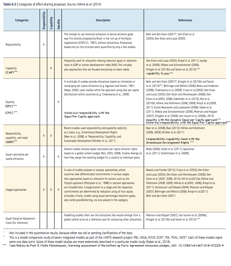
Categories of effort-sharing
Table 6.5. Categories of effort-sharing proposals (Source: Höhne N, M G J den Elzen, and D Escalante (2014). Regional GHG reduction targets based on effort sharing: a comparison of studies. Climate Policy 14, 122 – 147. doi: 10.1080 / 14693062.2014.849452.
zum Vergrößern auf Tabelle klicken
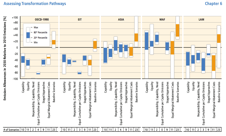
Figure 6.28: Emission allowances in 2030 relative to 2010 emissions by effort-sharing category for mitigation scenarios reaching 430 - 480 ppm CO2eq in 2100. GHG emissions (all gases and sectors) in GtCO2eq in 1990 and 2010 were
Emissions allowances are shown compared to 2010 levels, but this does not imply a preference for a specific base-year. For the OECD-1990 in the category 'responsibility, capability, need' the emission allowances in 2030 is - 106 % to - 128 % (20th to 80th percentile) below 2010 level (therefore not shown here). The studies with the 'Equal cumulative per capita emissions' approaches do not have the regional representation MAF. For comparison in orange: 'Equal marginal abatement cost' (allocation based on the imposition of a global carbon price) and baseline scenarios. Source: Adapted from Höhne et al.(2014). Studies were placed in this CO2eq concentration range based on the level that the studies themselves indicate. The pathways of the studies were compared with the characteristics of the range, but concentration levels were not recalculated.
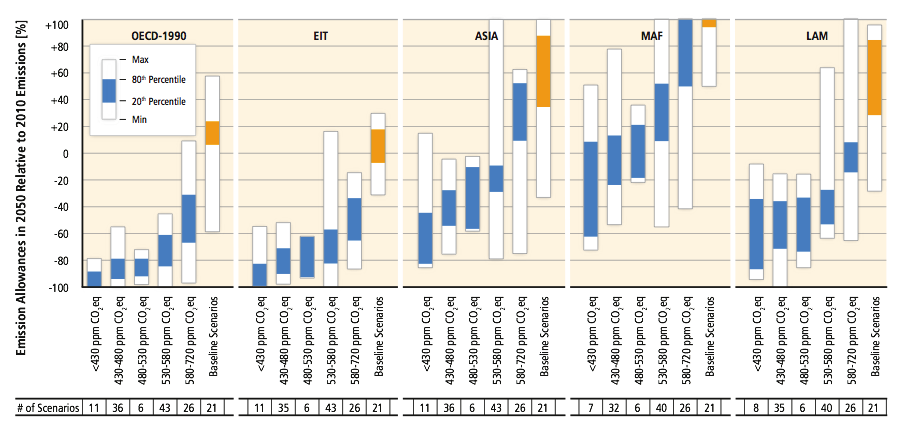
Figure 6.29: Emission allowances in 2050 relative to 2010 emissions for different 2100 CO2eq concentration ranges by all effort-sharing categories except 'equal marginal abate- ment costs'. For comparison in orange: baseline scenarios. Source: Adapted from Höhne et al. (2014). Studies were placed in the CO2eq concentration ranges based on the level that the studies themselves indicate. The pathways of the studies were compared with the characteristics of the ranges, but concentration levels were not recalculated.
/fig4.png)
zum Vergrößern auf Bild klicken
Fig.4 Global warming responses under the CBDR-RC hybrid approach following NDCs' ambitions. Global warming assessment(50% likelihood, compared with pre-industrial levels)of average NDC ambitions for 169 countries (maps with high and low NDC quantifications inSupplementary Figs. 9 and 10).
Quelle: Yann Robiou du Pont & Malte Meinshausen, Warming assessment of the bottom-up Paris Agreement emissions pledges, NATURE COMMUNICATIONS (2018) 9:4810 DOI: 10.1038/s41467-018-07223-9
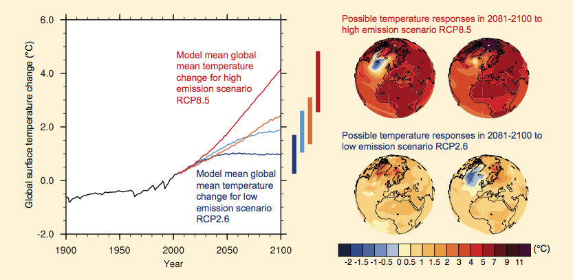
FAQ 12.1, Figure 1: Global mean temperature change averaged across all Coupled Model Intercomparison Project Phase 5 (CMIP5) models (relative to 1986 - 2005) for the four Representative Concentration Pathway (RCP) scenarios: RCP2.6 (dark blue), RCP4.5 (light blue), RCP6.0 (orange) and RCP8.5 (red); 32, 42, 25 and 39 models were used respectively for these 4 scenarios. Likely ranges for global temperature change by the end of the 21st century are indicated by vertical bars. Note that these ranges apply to the difference between two 20-year means, 2081 - 2100 relative to 1986 - 2005, which accounts for the bars being centred at a smaller value than the end point of the annual trajectories. For the highest (RCP8.5) and lowest (RCP2.6) scenario, illustrative maps of surface temperature change at the end of the 21st century (2081 - 2100 relative to 1986 - 2005) are shown for two CMIP5 models. These models are chosen to show a rather broad range of response, but this particular set is not representative of any measure of model response uncertainty.
Quelle: Seite 1037 in IPCC_WGI_AR5_all_final.pdf
An IPCC Special Report on the impacts of global warming of 1.5 °C above pre-industrial levels and related global greenhouse gas emission pathways, in the context of strengthening the global response to the threat of climate change, sustainable development, and efforts to eradicate poverty
pages 59, 60
Pathways considered in this report, consistent with available literature on 1.5 °C, primarily focus on the time scale up to 2100, recognising that the evolution of GMST after 2100 is also important. ... Because of uncertainty in the climate response, a 'prospective' mitigation pathway (see Cross-Chapter Box 1 in this chapter), in which emissions are prescribed, can only provide a level of probability of warming remaining below a temperature threshold. This probability cannot be quantified precisely since estimates depend on the method used (Rogelj et al., 2016b; Millar et al., 2017b; Goodwin et al., 2018; Tokarska and Gillett, 2018). ...
... All these absolute probabilities are
Imprecise probabilities can nevertheless be useful for decision-making, provided the imprecision is acknowledged (Hall et al., 2007; Kriegler et al., 2009; Simpson et al., 2016).
Relative and rank probabilities can be assessed much more consistently:
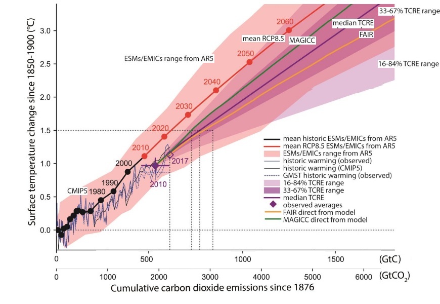
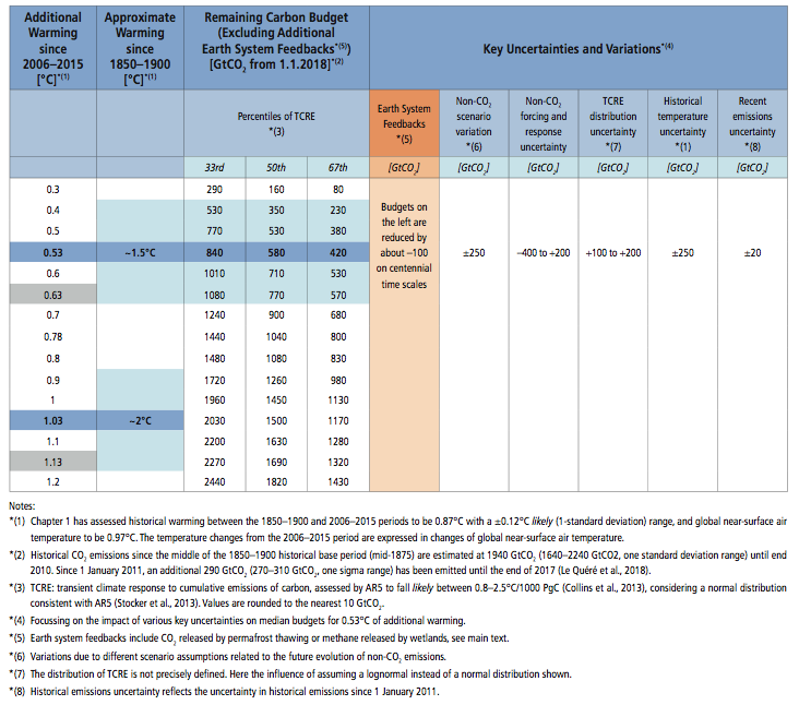
Figure 2.3: Temperature changes from 1850–1900 versus cumulative CO2 emissions since 1st January 1876. Solid lines with dots reproduce the globally averaged near-surface air temperature response to cumulative CO2 emissions plus non-CO2 forcers as assessed in Figure SPM10 of WGI AR5, except that points marked with years relate to a particular year, unlike in WGI AR5 Figure SPM.10, where each point relates to the mean over the previous decade. The AR5 data was derived from 15 Earth system models and 5 Earth system models of Intermediate Complexity for the historic observations (black) and RCP8.5 scenario (red), and the red shaded plume shows the range across the models as presented in the AR5. The purple shaded plume and the line are indicative of the temperature response to cumulative CO2 emissions and non-CO2 warming adopted in this report. The non-CO2 warming contribution is averaged from the MAGICC and FAIR models, and the purple shaded range assumes the AR5 WGI TCRE distribution (Supplementary Material 2.SM.1.1.2). The 2010 observation of surface temperature change (0.97°C based on 2006–2015 mean compared to 1850–1900, Chapter 1, Section 1.2.1) and cumulative carbon dioxide emissions from 1876 to the end of 2010 of 1,930 GtCO2 (Le Quéré et al., 2018) is shown as a filled purple diamond. The value for 2017 based on the latest cumulative carbon emissions up to the end of 2017 of 2,220 GtCO2 (Version 1.3 accessed 22 May 2018) and a surface temperature anomaly of 1.1°C based on an assumed temperature increase of 0.2°C per decade is shown as a hollow purple diamond. The thin blue line shows annual observations, with CO2 emissions from Le Quéré et al. (2018) and estimated globally averaged near-surface temperature from scaling the incomplete coverage and blended HadCRUT4 dataset in Chapter 1. The thin black line shows the CMIP5 multimodel mean estimate with CO2 emissions also from (Le Quéré et al., 2018). The thin black line shows the GMST historic trends from Chapter 1, which give lower temperature changes up to 2006–2015 of 0.87°C and would lead to a larger remaining carbon budget. The dotted black lines illustrate the remaining carbon budget estimates for 1.5°C given in Table 2.2. Note these remaining budgets exclude possible Earth system feedbacks that could reduce the budget, such as CO2 and CH4 release from permafrost thawing and tropical wetlands (see Section 2.2.2.2)
Table 2.2 The assessed remaining carbon budget and its uncertainties. Shaded blue horizontal bands illustrate the uncertainty in historical temperature increase from the 1850–1900 base period until the 2006–2015 period as estimated from global near-surface air temperatures, which impacts the additional warming until a specific temperature limit like 1.5°C or 2°C relative to the 1850–1900 period. Shaded grey cells indicate values for when historical temperature increase is estimated from a blend of near-surface air temperatures over land and sea ice regions and sea-surface temperatures over oceans.
Sources
IPCC-SR15
IPCC WG3 AR5, Seiten 1249 ff
|
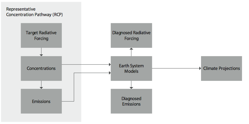
Figure 12.2: Links in the chain from scenarios, through models to climate projections. The Representative Concentration Pathways (RCPs) are designed to sample a range of radiative forcing (RF) of the climate system at 2100. The RCPs are translated into both concentrations and emissions of greenhouse gases using Integrated Assessment Models (IAMs). These are then used as inputs to dynamical Earth System Models (ESMs) in simulations that are either concentration-driven (the majority of projection experiments) or emissions-driven (only for RCP8.5). Aerosols and other forcing factors are implemented in different ways in each ESM. The ESM projections each have a potentially different RF, which may be viewed as an output of the model and which may not correspond to precisely the level of RF indicated by the RCP nomenclature. Similarly, for concentration-driven experiments, the emissions consistent with those concentrations diagnosed from the ESM may be different from those specified in the RCP (diagnosed from the IAM). Different models produce different responses even under the same RF. Uncertainty propagates through the chain and results in a spread of ESM projections. This spread is only one way of assessing uncertainty in projections. Alternative methods, which combine information from simple and complex models and observations through statistical models or expert judgement, are also used to quantify that uncertainty.
The ability of models to mimic nature is achieved by simplification choices that can vary from model to model in terms of the fundamental numeric and algorithmic structures, forms and values of parameterizations, and number and kinds of coupled processes included. Simplifications and the interactions between parameterized and resolved processes induce "errors" in models, which can have a leading-order impact on projections. It is possible to characterize the choices made when building and running models into structural - indicating the numerical techniques used for solving the dynamical equations, the analytic form of parameterization schemes and the choices of inputs for fixed or varying boundary conditions - and parametric - indicating the choices made in setting the parameters that control the various components of the model. (Quelle: Seite 1039 von IPCC_WGI_AR5_all_final.pdf |
Global mean surface temperature (GMST)
Estimated global average of near-surface air temperatures over land and sea-ice, and sea surface temperatures over ice-free ocean regions, with changes normally expressed as departures from a value over a specified reference period. When estimating changes in GMST, near-surface air temperature over both land and oceans are also used. 1 See also Land surface air temperature, Sea surface temperature (SST) and Global mean surface air temperature (GSAT).
Global mean surface air temperature (GSAT) Global average of near-surface air temperatures over land and oceans. Changes in GSAT are often used as a measure of global temperature change in climate models but are not observed directly. See also Land surface air temperature. Land surface air temperature The near-surface air temperature over land, typically measured at 1.25 cm above the ground using standard meteorological equipment. Sea surface temperature (SST) The sea surface temperature is the subsurface bulk temperature in the top few meters of the ocean, measured by ships, buoys, and drifters. From ships, measurements of water samples in buckets were mostly switched in the 1940s to samples from engine intake water. Satellite measurements of skin temperature (uppermost layer; a fraction of a millimeter thick) in the infrared or the top centimeter or so in the microwave are also used, but must be adjusted to be compatible with the bulk temperature.
Global warming The expressed relative to pre-industrial levels unless otherwise specified. For 30-year periods that span past and future years, the current multi-decadal warming trend is assumed to continue. See also Climate change and Climate variability. Integrated assessment model (IAM) Integrated assessment models (IAMs) integrate knowledge from two or more domains into a single framework. They are one of the main tools for undertaking integrated assessments.
One class of IAM used in respect of climate change mitigation may include representations of
This class of model is used to assess linkages between economic, social and technological development and the evolution of the climate system.
Another class of IAM additionally includes representations of the costs associated with climate change impacts, but includes less detailed representations of economic systems. These can be used to assess impacts and mitigation in a cost-benefit framework and have been used to estimate the social cost of carbon. Atmosphere–ocean general circulation model (AOGCM) A numerical representation of the climate system based on the physical, chemical and biological properties of its components, their interactions and feedback processes, and accounting for some of its known properties. The climate system can be represented by models of varying complexity; that is, for any one component or combination of components a spectrum or hierarchy of models can be identified, differing in such aspects as the number of spatial dimensions, the extent to which physical, chemical or biological processes are explicitly represented, or the level at which empirical parametrizations are involved. There is an evolution towards more complex models with interactive chemistry and biology. Climate models are applied as a research tool to study and simulate the climate and for operational purposes, including monthly, seasonal and interannual climate predictions. See also Earth system model (ECS). Earth system model (ESM) A coupled atmosphere–ocean general circulation model in which a representation of the carbon cycle is included, allowing for interactive calculation of atmospheric CO2 or compatible emissions. Additional components (e.g., atmospheric chemistry, ice sheets, dynamic vegetation, nitrogen cycle, but also urban or crop models) may be included. Carbon cycle: The term used to describe the flow of carbon (in various forms, e. g., as carbon dioxide) through the atmosphere, ocean, terrestrial and marine biosphere and lithosphere. In this report, the reference unit for the global carbon cycle is GtC or GtCO2 (1 GtC corresponds to 3.667 GtCO2). Carbon is the major chemical constituent of most organic matter and is stored in the following major reservoirs: organic molecules in the biosphere, carbon dioxide (CO2) in the atmosphere, organic matter in the soils, in the lithosphere, and in the oceans. CIMP5: The CMIP5 multi-model experiment (coordinated through the World Climate Research Programme) presents an unprecedented level of
information on which to base assessments of climate variability and change. CMIP5 includes new ESMs in addition to AOGCMs, new
model experiments and more diagnostic output. CMIP5 is much more comprehensive than the preceding CMIP3 multi-model experiment that was available at the time of the IPCC AR4. CMIP5 has more than twice as many models, many more experiments (that also
include experiments to address understanding of the responses in the future climate change scenario runs), and nearly 2 x 1015 bytes
of data (as compared to over 30 x 1012 bytes of data in CMIP3). A larger number of forcing agents are treated more completely in the
CMIP5 models, with respect to aerosols and land use particularly. Black carbon aerosol is now a commonly included forcing agent.
Considering CO2, both ‘concentrations-driven’ projections and ‘emissions-driven’ projections are assessed from CMIP5. These allow
quantification of the physical response uncertainties as well as climate–carbon cycle interactions. {1.5.2}
The assessment of the mean values and ranges of global mean temperature changes in AR4 would not have been substantially different if the CMIP5 models had been used in that report. The differences in global temperature projections can largely be attributed
to the different scenarios. The global mean temperature response simulated by CMIP3 and CMIP5 models is very similar, both in the
mean and the model range, transiently and in equilibrium. The range of temperature change across all scenarios is wider because the
RCPs include a strong mitigation scenario (RCP2.6) that had no equivalent among the SRES scenarios used in CMIP3. For each scenario,
the 5 to 95% range of the CMIP5 projections is obtained by approximating the CMIP5 distributions by a normal distribution with
same mean and standard deviation and assessed as being likely for projections of global temperature change for the end of the 21st
century. Probabilistic projections with simpler models calibrated to span the range of equilibrium climate sensitivity assessed by the
AR4 provide uncertainty ranges that are consistent with those from CMIP5. In AR4 the uncertainties in global temperature projections
were found to be approximately constant when expressed as a fraction of the model mean warming (constant fractional uncertainty).
For the higher RCPs, the uncertainty is now estimated to be smaller than with the AR4 method for long-term climate change, because
the carbon cycle–climate feedbacks are not relevant for the concentration-driven RCP projections (in contrast, the assessed projection
uncertainties of global temperature in AR4 did account of carbon cycle–climate feedbacks, even though these were not part of the
CMIP3 models). When forced with RCP8.5, CO2 emissions, as opposed to the RCP8.5 CO2 concentrations, CMIP5 ESMs with interactive
carbon cycle simulate, on average, a 50 (-140, +210) ppm (CMIP5 model spread) larger atmospheric CO2 concentration and 0.2°C
larger global surface temperature increase by 2100. For the low RCPs the fractional uncertainty is larger because internal variability and
non-CO2 forcings make a larger relative contribution to the total uncertainty. {12.4.1, 12.4.8, 12.4.9}
There is overall consistency between the projections of temperature and precipitation based on CMIP3 and CMIP5, both for large-scale
patterns and magnitudes of change (Box TS.6, Figure 1). Model agreement and confidence in projections depends on the variable and
on spatial and temporal averaging, with better agreement for larger scales. Confidence is higher for temperature than for those quantities related to the water cycle or atmospheric circulation. Improved methods to quantify and display model robustness have been
developed to indicate where lack of agreement across models on local trends is a result of internal variability, rather than models actually disagreeing on their forced response. Understanding of the sources and means of characterizing uncertainties in long-term large
scale projections of climate change has not changed significantly since AR4, but new experiments and studies have continued to work
towards a more complete and rigorous characterization. {9.7.3, 12.2, 12.4.1, 12.4.4, 12.4.5, 12.4.9; Box 12.1}
The well-established stability of geographical patterns of temperature and precipitation change during a transient experiment remains
valid in the CMIP5 models (Box TS.6, Figure 1). Patterns are similar over time and across scenarios and to first order can be scaled by
the global mean temperature change. There remain limitations to the validity of this technique when it is applied to strong mitigation
scenarios, to scenarios where localized forcings (e.g., aerosols) are significant and vary in time and for variables other than average
seasonal mean temperature and precipitation. {12.4.2} Climate: Climate in a narrow sense is usually defined as the average weather, or more rigorously, as the statistical description in terms of the mean and variability of relevant quantities over a period of time ranging from months to thousands or millions of years. The classical period for averaging these variables is 30 years, as defined by the World Meteorological Organization. The relevant quantities are most often surface variables such as temperature, precipitation and wind. Climate in a wider sense is the state, including a statistical description, of the climate system. Climate model (spectrum or hierarchy): A numerical representation of the climate system based on the physical, chemical and biological properties of its components, their interactions and feedback processes, and accounting for some of its known properties. The climate system can be represented by models of varying complexity, that is, for any one component or combination of components a spectrum or hierarchy of models can be identified, differing in such aspects as the number of spatial dimensions, the extent to which physical, chemical or biological processes are explicitly represented, or the level at which empirical parametrizations are involved. Coupled Atmosphere-Ocean General Circulation Models (AOGCMs) provide a representation of the climate system that is near or at the most comprehensive end of the spectrum currently available. There is an evolution towards more complex models with interactive chemistry and biology. Climate models are applied as a research tool to study and simulate the climate, and for operational purposes, including monthly, seasonal and interannual climate predictions. Climate system: The climate system is the highly complex system consisting of five major components: the atmosphere, the hydrosphere, the cryosphere, the lithosphere and the biosphere, and the interactions between them. The climate system evolves in time under the influence of its own internal dynamics and because of external forcings such as volcanic eruptions, solar variations and anthropogenic forcings such as the changing composition of the atmosphere and land use change (LUC). CO2-equivalent emission: The amount of carbon dioxide (CO2) emission that would cause the same integrated radiative forcing, over a given time horizon, as an emitted amount of a greenhouse gas (GHG) or a mixture of GHGs. The CO2-equivalent emission is obtained by multiplying the emission of a GHG by its Global Warming Potential (GWP) for the given time horizon (see Annex II.9.1 and WGI AR5 Table 8.A.1 for GWP values of the different GHGs). For a mix of GHGs it is obtained by summing the CO2-equivalent emissions of each gas. CO2-equivalent emission is a common scale for comparing emissions of different GHGs but does not imply equivalence of the corresponding climate change responses..
Coupled Model Intercomparison Project (CMIP)
The Coupled Model Intercomparison Project (CMIP) is a climate modelling activity from the World Climate Research Programme (WCRP) which coordinates and archives climate model simulations based on shared model inputs by modelling groups from around the world. The CMIP3 multimodel data set includes projections using SRES scenarios. The CMIP5 data set includes projections using the Representative Concentration Pathways (RCPs). The CMIP6 phase involves a suite of common model experiments as well as an ensemble of CMIP-endorsed model intercomparison projects (MIPs).
Emission quota: The portion of total allowable emissions assigned to a country or group of countries within a framework of maximum total emissions.
Global mean surface temperature (GMST): An estimate of the global mean surface air temperature. However, for changes over time, only anomalies, as departures from a climatology, are used, most commonly based on the area-weighted global average of the sea surface temperature anomaly and land surface air temperature anomaly.
Global warming: Global warming refers to the gradual increase, observed or projected, in global surface temperature, as one of the consequences of radiative forcing caused by anthropogenic emissions.
Human Development Index (HDI): The Human Development Index allows the assessment of countries’ progress regarding social and economic development as a composite index of three indicators: (1) health measured by life expectancy at birth; (2) knowledge as measured by a combination of the adult literacy rate and the combined primary, secondary and tertiary school enrolment ratio; and (3) standard of living as gross domestic product (GDP) per capita (in purchasing power parity). The HDI sets a minimum and a maximum for each dimension, called goalposts, and then shows where each country stands in relation to these goalposts, expressed as a value between 0 and 1. The HDI only acts as a broad proxy for some of the key issues of human development; for instance, it does not reflect issues such as political participation or gender inequalities.
Models: Structured imitations of a system’s attributes and mechanisms to mimic appearance or functioning of systems, for example, the climate, the economy of a country, or a crop. Mathematical models assemble (many) variables and relations (often in a computer code) to simulate system functioning and performance for variations in parameters and inputs.
Computable General Equilibrium (CGE) Model: A class of economic models that use actual economic data (i. e., input / output data), simplify the characterization of economic behaviour, and solve the whole system numerically. CGE models specify all economic relationships in mathematical terms and predict the changes in variables such as prices, output and economic welfare resulting from a change in economic policies, given information about technologies and consumer preferences (Hertel, 1997).
Representative Concentration Pathways (RCPs): Scenarios that include time series of emissions and concentrations of the full suite of greenhouse gases (GHGs) and aerosols and chemically active gases, as well as land use / land cover (Moss et al., 2008). The word representative signifies that each RCP provides only one of many possible scenarios that would lead to the specific radiative forcing characteristics. The term pathway emphasizes that not only the long-term concentration levels are of interest, but also the trajectory taken over time to reach that outcome (Moss et al., 2010).
RCPs usually refer to the portion of the concentration pathway extending up to 2100, for which Integrated Assessment Models produced corresponding emission scenarios. Extended Concentration Pathways (ECPs) describe extensions of the RCPs from 2100 to 2500 that were calculated using simple rules generated by stakeholder consultations, and do not represent fully consistent scenarios.
Four RCPs produced from Integrated Assessment Models were selected from the published literature and are used in the present IPCC Assessment as a basis for the climate predictions and projections presented in WGI AR5 Chapters 11 to 14:
Equilibrium climate sensitivity (ECS)
refers to the equilibrium (steady state) change in the annual global mean surface temperature following a doubling of the atmospheric carbon dioxide (CO2) concentration. As a true equilibrium is challenging to define in climate models with dynamic oceans, the equilibrium climate sensitivity is often estimated through experiments in AOGCMs where CO2 levels are either quadrupled or doubled from pre-industrial levels and which are integrated for 100-200 years. The climate sensitivity parameter (units: °C (W m–2)–1) refers to the equilibrium change in the annual global mean surface temperature following a unit change in radiative forcing.
The transient climate response to cumulative CO2 emissions (TCRE)
is the ratio between globally averaged surface temperature increase and cumulative CO2 emissions.
This report (IPCC WG1 AR6) reaffirms with high confidence the finding of AR5 that there is a near-linear relationship between cumulative CO2 emissions and the increase in global average temperature caused by CO2 over the course of this century for global warming levels up to at least 2°C relative to 1850–1900.
The TCRE falls likely in the 1.0°C–2.3°C per 1000 PgC range, with a best estimate of 1.65°C per 1000 PgC. This range is about 15% narrower than the 0.8°–2.5°C per 1000 PgC assessment of the AR5 because of a better integration of evidence across chapters, in particular the assessment of TCR.
Beyond this century, there is low confidence that the TCRE alone remains an accurate predictor of temperature changes in scenarios of very low or net negative CO2 emissions because of uncertain Earth system feedbacks that can result in further changes in temperature or a path dependency of warming as a function of cumulative CO2 emissions. {5.4, 5.5.1, 4.6.2}
Version: 8.11.2021
Adresse dieser Seite
Home
Joachim Gruber